WELL-LOG DIGITIZING, PLOTTING & CORRELATION

Digitize well logs
Make correlation charts

Bring scanned and digital well logs into one browser workspace. Trace calibrated curves from scans, or import LAS, Excel and CSV files. Build log displays, pick formation tops and correlate wells in LogPlot Studio, then export your curves, tops and charts.

From PDF and TIFF scans to LAS, Excel and CSV data Curve tracing · Custom tracks · Formation tops · Well correlation

01—03

Watch the workflow on the right.
Load, calibrate, trace and export.

MAP STUDIO · FROM SCAN TO MAP

Old maps on paper?
Make them working maps.

Structure and isopach maps often survive only as prints. Map Studio gives the scan real coordinates, lets you trace its faults and contours with their values, and turns them into a finished map you can edit, print or take into other software.

Open Map Studio

LOGPLOT STUDIO

Build log displays
and correlate wells

Drop LAS, Excel, CSV or text files into the workspace, or send in the curves you just digitized. Start with a triple-combo layout, then shape the log around your work.

  • Drag curves between tracks; insert and resize tracks.
  • Change scales, line styles and fills—including fills between two curves.
  • Pick formation tops on the log and drag their depths to refine them.
  • Open multiple wells, pick and adjust tops on the correlation chart, and flatten on a chosen datum.
  • Choose lithology fills and FGDC patterns; inspect coverage, spikes and borehole-quality checks.
  • Start from templates or saved layouts; use publication presets and vector PDF with searchable text.
  • Reopen your Studio session from your auto-save folder, then export plot PDFs or correlation slides for PowerPoint.
Open Log Digitize workspace

In the workspace, choose File → LogPlot Studio.

Explore the studio

Synthetic preview

Three curve tracks share a depth axis. In the full studio, drag curve headers to arrange your sheet.

Illustrative data. The full studio uses your imported or digitized curves.

LOGPLOT STUDIO · EVALUATION

Evaluate your logs
with charts and statistics

Once your curves are in LogPlot Studio, open Charts to look at the rock, not just the curves. Compare wells and formation zones side by side, with the numbers beside every plot.

  • Crossplots with neutron–density, Pickett and M–N chart overlays, coloured by zone or by a third curve.
  • Histograms with mean, P10, P50 and P90 for each well or zone, and a bin size you control.
  • Box plots with median, quartiles, whiskers, IQR and outliers.
  • Change the colour of any histogram or box, and filter by interval or by formation tops.
Open Log Digitize workspace

In the workspace, choose Charts in the toolbar (or press G).

Explore the charts

Synthetic preview

Illustrative data. The Charts window uses your imported or digitized curves.

A CLEAR PATH FROM SCAN TO EXPORT

Digitize a scanned log
in six guided steps

Start with the guided sample, then use the same workflow on your own logs. The tour highlights the next tool and can be skipped at any time.

Explore the guided sample
01Open a scan and select an interval

Upload a PDF, TIFF, or image. Pick the top and bottom on the overview, then load the selected interval with more detail. For multi-page PDFs, choose the page you need.

02Calibrate the depth

Enter two known depths and pick their horizontal marks on the scan. Use feet or metres. Depth ties and breaks are available in Advanced tools.

03Calibrate each curve

Add a curve beneath Curve calibration. Start with a new track and depth, or copy from another curve. Enter its left and right values, pick the track edges, and choose a linear or logarithmic scale. Resistivity commonly uses a logarithmic scale.

04Trace curves and refine your points

Use the Pen to click an anchor or draw a smooth stroke along the curve. Right-click on the printed curve for automatic tracing. In Trace mode, completed intervals stay protected as you extend the curve. Choose Select anchors to click or box-select points, move them together, or delete them. A new Pen stroke replaces only its depth span; Undo restores the previous trace.

05Review and correct a section

In Advanced tools, select a rectangle, choose a seed point, and preview a local trace. Edit the preview before applying it. Inspect crossings, faded ink, and grid lines before exporting.

06Export data and save your project

Send digitized curves to LogPlot Studio to plot them alongside imported data. Select individual curves or all curves. Export LAS or CSV at your chosen depth interval; Excel and text are available in Advanced tools. Export defaults to the traced interval. Untraced depths stay null. Save a project file to resume later.

MAP STUDIO

Digitize or import maps.
Edit contours. Export.

Map Studio turns scanned maps into editable contours, faults, boundaries and well locations, or starts from your own data: import points, contour lines or grids, refine the contours, and export them in the format you need. Set real-world coordinates, organize your work into layers, and fill geological areas with colors and sedimentary patterns.

  • Import map data: XYZ, CSV and text points; contour lines (Irap, CPS, GMT, GeoJSON); and grids (ZMAP+, Surfer ASCII, Esri ASCII, GRASS, Irap). Grids and points become contours at the interval you choose, on your georeferenced map or on a new base map sized to the data.
  • Modify contours: move, add or delete vertices, smooth, simplify, join, cut, offset, blend and relabel depths, then check for open, duplicate or crossing contours.
  • Georeference from control points, and search all EPSG reference systems.
  • Pen tools for contours (with depth), faults, boundaries and well locations.
  • Choose Trace, click a printed line, and accept the preview as a contour, fault or boundary.
  • Fill boundaries with Shale, Dolomite, Sandstone, Anhydrite, Limestone, Conglomerate and more stratigraphic patterns.
  • Create your own named feature layers, with visibility and locking controls.
  • Add wells by clicking, by typed coordinates, or by importing a CSV.
  • Select and edit vertices; erase any feature; undo and redo.
  • Illustrator-style editing: Scissors, Join, Smooth, Simplify, Offset, Blend between contours, Clip to a boundary, Rotate, Scale, Flip, Align, Group, Lock, an Eyedropper to copy a look, fault ticks, and labels that run along a line.
  • Drag layers into stacking order (like Illustrator), right-click for Close, Depth and more, and save or reopen your map project.
  • Make a finished map: add a title, legend, scale bar, north arrow and coordinate labels, then download it as SVG (opens in Illustrator), PNG or PDF.
  • Export by layer or all together: CSV, GeoJSON, XYZ, Shapefile, DXF, KML, GPX, WKT, SVG, GMT, GOCAD TSurf, Irap and gridded ZMAP, Surfer, Esri ASCII and GRASS — in the map’s coordinates or any EPSG system.
Open Map Studio

Open a map, a saved project, or Open ▾ → Surface data to import points, contours or grids.
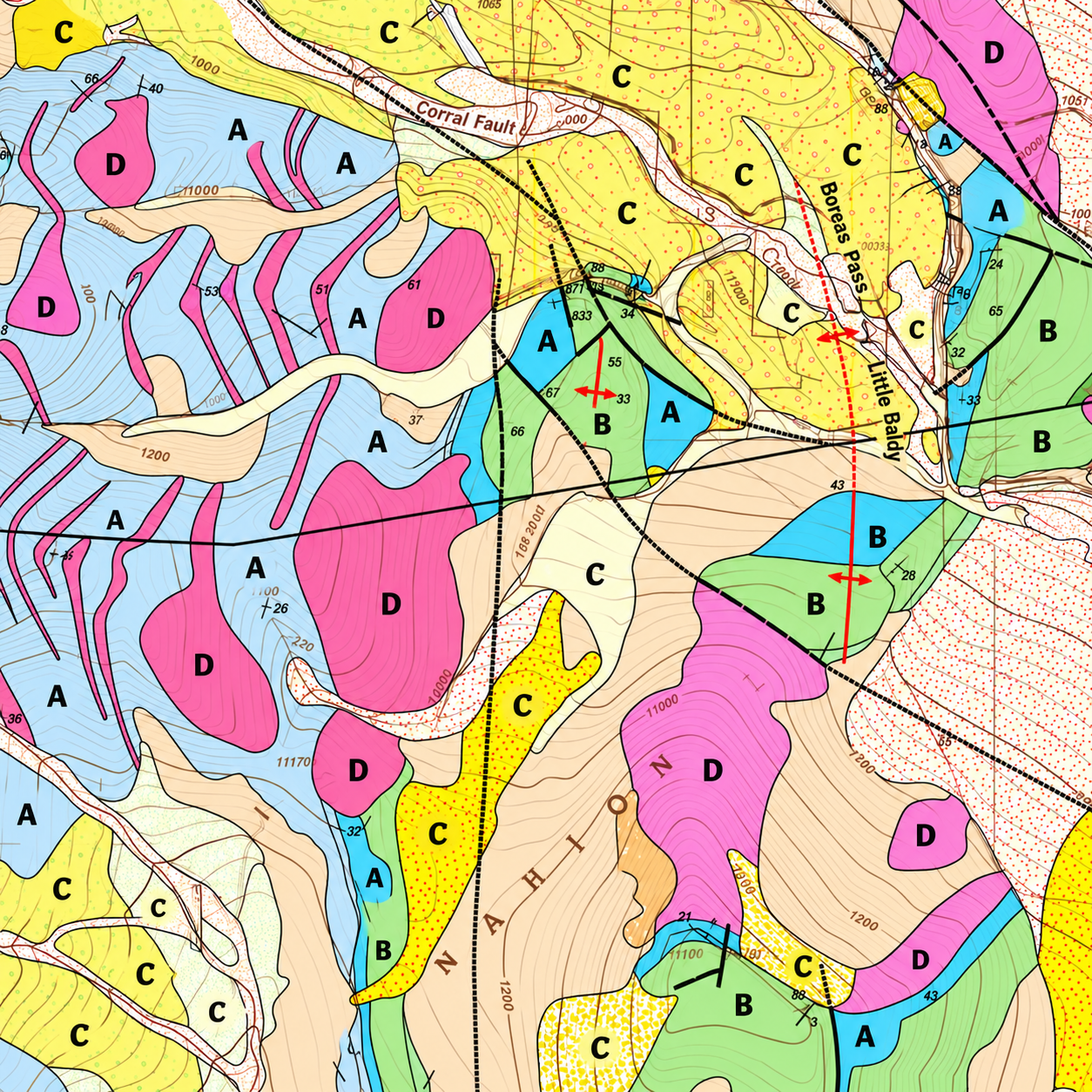
Maps, colors & patterns

Geological map
Colorful geological map showing formation boundaries, faults, contours and lithologic patterns

Digitize your own maps or import map data, edit the contours, and style geological areas with colors and stratigraphic patterns. Your maps stay on your computer.

BUILT AROUND THE WAY YOU WORK

Tools for every stage
of your well-log workflow

/01

A focused workspace

Depth, curve calibration, tracing, and export stay within reach. Techlog-inspired menus and Advanced tools bring out more options when you need them.

/02

Assistance you can review

Right-click tracing, color-based tracing, and local section previews speed up the work. Edit points and Undo give you the final say.

/03

Curves on their own terms

Set independent depths, track edges, units, and scales. Delete a digitized curve while keeping the original raster and your other curves.

/04

Data ready for your next step

Send traced curves into LogPlot Studio, or import existing well-log data. Export curves and formation tops as LAS or CSV, save a full-length plot as PNG, or print your log sheet.

Everything in the workspace

Five tools, one private workspace: digitize, plot and correlate, map, and export.

01Digitize

Digitize scanned logs

  • Open PDF, TIFF, PNG, JPEG or WebP scans; choose a page of a multi-page PDF, select an interval on the overview, then load it in detail. Straighten a tilted scan.
  • Calibrate depth in feet or metres from two known marks, with depth ties, breaks and backup intervals.
  • Calibrate every curve on its own: track edges, linear or logarithmic scale, units and backup scales.
  • Trace with the Pen (snaps to the ink), right-click auto-tracing, color-based tracing and guided resume; preview a local section before you apply it.
  • Select anchors one by one or by box, move or delete them together, erase, and Undo / Redo every step.
  • Review crossings, faded ink and grid lines; run data checks; compare your trace with a LAS file; try the sample log and guided tour.
02Export

Export and exchange data

  • Export LAS 2.0, LAS 3.0, CSV, Excel and tab-separated text at the depth interval you choose; untraced depths stay null.
  • Measured depth or subsea (with KB), formation tops as CSV, a QC image and a data table view.
  • Convert LAS, Excel, CSV, TSV and text data files, or open them in LogPlot Studio.
  • Save projects (.strata) and keep working later; save to a folder on your computer with automatic saving (Chrome or Edge).
03Plot & correlate

LogPlot Studio

  • Start from API, triple-combo, quad-combo, petrophysical or geological templates and save your own layouts.
  • Arrange tracks and curves by dragging; set scales, line styles, fonts and fills, including fills between curves.
  • Lithology fills with 117 FGDC patterns and neutron–density, PE and gamma-ray lithology classes; QC for coverage, spikes and bad hole.
  • Annotate with arrows, lines (optional arrowheads and distance label), unconformity and fault marks that can cross between wells.
  • Pick formation tops, drag them to refine, open several wells and correlate on a flattened datum.
  • Export PNG (up to 4×), vector PDF with searchable text (Letter, A4 or custom size), PowerPoint correlation slides and print; publication presets with journal column widths.
04Privacy

Private, saved, yours

  • PDF and image processing runs in your browser; your logs and maps stay on your computer.
  • Auto-save to a folder you choose, with unsaved-work recovery.
  • Save project asks whether to replace the file you opened or keep it and save a new version.
  • Built-in illustrated guides, keyboard shortcuts and a Send feedback form; free log to start, then pay per log or map, or choose three-month or annual access.
05Maps

Map Studio

  • Georeference a scanned map from three control points and search all EPSG coordinate systems.
  • Trace printed lines with one click, or draw contours (with depth), faults, boundaries, wells and text labels; right-click for Close, Depth, Auto-trace and Smooth.
  • Measure distances, show a coordinate grid, assign depths and check contours.
  • Edit lines like in Illustrator: cut with Scissors, Join or close, Smooth, Simplify, add or delete anchors, Offset a parallel copy, Blend new contours between two, Reverse, and Clip lines to a boundary.
  • Transform, align and distribute; group, lock and hide; fault ticks and thrust triangles; labels that follow a line; copy and paste a look with the Eyedropper.
  • Organize named layers: show, hide, lock and drag them into stacking order like Illustrator; fill boundaries with colors and stratigraphic patterns.
  • Open a map image or PDF; it is read in your browser and never uploaded. Fit, pan and zoom, with a keyboard shortcut for every tool.
  • Draw contours with a depth or elevation, fault traces, boundaries and polygons, well locations and text labels; click a contour to enter its depth.
  • Check your work: find open, duplicate or crossing contours, see the misfit at each control point, and Undo / Redo every step.
  • Save the project (.strata) together with your map work and reopen it later.
  • Export by layer or all together as CSV, GeoJSON, XYZ, Shapefile, DXF, KML, GPX, WKT, SVG, GMT, GOCAD TSurf, Irap and gridded ZMAP, Surfer, Esri ASCII or GRASS.

Bring in

PDF, TIFF, PNG, JPEG, WebP
LAS, Excel, CSV, TSV and text data

Take out

LAS, CSV, Excel, text
Log sheets as PNG or PDF
PowerPoint correlation slides and projects

Keep in mind

PDF and image processing runs in your browser. Review calibration and tracing before interpretation.

CHOOSE WHAT FITS YOUR WORK

Choose access for your project

Start with one free log per account. For more work, pay per log or map, or choose three-month or annual access.

START FREE

Free account

$0 / account

One free log per user account.

  • One log total, including its curves and intervals
  • Calibration, tracing, and review tools
  • LogPlot Studio access to plot and export the log you digitize
  • Corrections and repeat LAS / CSV exports
  • Map Studio exports need a purchased map or a paid plan
Create free account

No card needed · start right away

OCCASIONAL USE

Per log or map

$10 / log or map

Buy exactly what you need: choose how many logs and how many maps. Each is $10.

Logs
Maps
$101 log × $10
  • Each map digitized in Map Studio is its own $10 purchase, with repeat exports of that map included
  • All curves in one scanned logging run
  • LogPlot Studio access for every log you digitize
  • Five additional data-file imports per raster log purchased
  • Its pages and selected intervals
  • Corrections and repeat LAS / CSV exports
Pay with card

Card, Apple Pay or Google Pay · secure checkout by Stripe

PROJECT ACCESS

Three months

$100 / 3 months

For a focused digitizing project. Map Studio is available.

  • Three months of full workspace access, including LogPlot Studio and Map Studio
  • Depth and curve calibration tools
  • Tracing, review, and export tools
Pay with card

Card, Apple Pay or Google Pay · secure checkout by Stripe

YEAR-ROUND ACCESS

Annual

$300 / year

For ongoing digitizing work. Map Studio is available.

  • One year of full workspace access, including LogPlot Studio and Map Studio
  • The same calibration and tracing tools
  • Save $100 versus four three-month plans
Pay with card

Card, Apple Pay or Google Pay · secure checkout by Stripe

Free accounts include five imported data logs plus one scanned log total. The allowance does not renew monthly. What counts as one log? One scanned logging run for one well, including its pages, intervals, and curves. Corrections and repeat exports of that log are included.

All prices are in USD. Payment is by card (or Apple Pay / Google Pay) on Stripe’s secure checkout; Log Digitize never sees your card details. Full refund within 14 days if the purchase has not been used — see the Terms and Privacy Policy. Three-month and annual access can be managed or cancelled from your account. The free log is used the first time you export a log; corrections and repeat exports of that log stay free.

YOUR NEXT LOG STARTS HERE

Start with a scan
or digital well data

Explore the digitizing sample, open a scan, or drop in existing log data. Use LogPlot Studio to arrange tracks and correlate wells.

Before you begin

Do I need to install anything?

No installation is needed. Log Digitize runs in your browser. Open the sample to learn the tools before bringing in a scan.

Does sign-in sync my logs between computers?

Sign-in controls workspace access. Your logs are never stored on the website or in the browser. Projects and Studio sessions are saved only in the folder you choose on your computer or in files you download; copy that folder or open a project file on another computer to continue.

Can I use LAS or Excel without digitizing a scan?

Yes. In File → LogPlot Studio, open LAS, Excel, CSV or text data. Select curves, edit their tracks and scales, add tops and export. Open two or more wells to use the correlation chart.

Can I trace upward as well as downward?

Yes. You can resume in either direction. Automatic continuation in Trace mode protects the interval you already traced. Draw a new Pen stroke when you want to replace a section; only that stroke’s depth span changes.

How are gaps exported?

Exports interpolate between traced points at the spacing you choose. Untraced depths remain null. Enable gap limits when you need to preserve intentional breaks; LAS and CSV use −999.25 for missing values.